
Regression metrics
Regression models have continuous output. So, we need a metric based on calculating some sort of distance between predicted and ground truth.
In order to evaluate Regression models, we’ll discuss these metrics in detail:
- Mean Absolute Error (MAE),
- Mean Squared Error (MSE),
- Root Mean Squared Error (RMSE),
- R² (R-Squared).
Mean Squared Error (MSE)
Mean squared error is perhaps the most popular metric used for regression problems. It essentially finds the average of the squared difference between the target value and the value predicted by the regression model.
Where:
- y_j: ground-truth value
- y_hat: predicted value from the regression model
- N: number of datums

Few key points related to MSE:
- It’s differentiable, so it can be optimized better.
- It penalizes even small errors by squaring them, which essentially leads to an overestimation of how bad the model is.
- Error interpretation has to be done with squaring factor(scale) in mind. For example in our Boston Housing regression problem, we got MSE=21.89 which primarily corresponds to (Prices)².
- Due to the squaring factor, it’s fundamentally more prone to outliers than other metrics.
This can be implemented simply using NumPy arrays in Python.
mse = (y-y_hat)**2
print(f"MSE: {mse.mean():0.2f} (+/- {mse.std():0.2f})")
Mean Absolute Error (MAE)
Mean Absolute Error is the average of the difference between the ground truth and the predicted values. Mathematically, its represented as :
Where:
- y_j: ground-truth value
- y_hat: predicted value from the regression model
- N: number of datums

Few key points for MAE
- It’s more robust towards outliers than MAE, since it doesn’t exaggerate errors.
- It gives us a measure of how far the predictions were from the actual output. However, since MAE uses absolute value of the residual, it doesn’t give us an idea of the direction of the error, i.e. whether we’re under-predicting or over-predicting the data.
- Error interpretation needs no second thoughts, as it perfectly aligns with the original degree of the variable.
- MAE is non-differentiable as opposed to MSE, which is differentiable.
Similar to MSE, this metric is also simple to implement.
mae = np.abs(y-y_hat)
print(f"MAE: {mae.mean():0.2f} (+/- {mae.std():0.2f})")
Root Mean Squared Error (RMSE)
Root Mean Squared Error corresponds to the square root of the average of the squared difference between the target value and the value predicted by the regression model. Basically, sqrt(MSE). Mathematically it can be represented as:
It addresses a few downsides in MSE.
Few key points related to RMSE:
- It retains the differentiable property of MSE.
- It handles the penalization of smaller errors done by MSE by square rooting it.
- Error interpretation can be done smoothly, since the scale is now the same as the random variable.
- Since scale factors are essentially normalized, it’s less prone to struggle in the case of outliers.
Implementation is similar to MSE:
mse = (y-y_hat)**2
rmse = np.sqrt(mse.mean())
print(f"RMSE: {rmse:0.2f}")
R² Coefficient of determination
R² Coefficient of determination actually works as a post metric, meaning it’s a metric that’s calculated using other metrics.
The point of even calculating this coefficient is to answer the question “How much (what %) of the total variation in Y(target) is explained by the variation in X(regression line)”
This is calculated using the sum of squared errors. Let’s go through the formulation to understand it better.
Total variation in Y (Variance of Y):
Percentage of variation described the regression line:

Subsequently, the percentage of variation described the regression line:

Finally, we have our formula for the coefficient of determination, which can tell us how good or bad the fit of the regression line is:

This coefficient can be implemented simply using NumPy arrays in Python.
# R^2 coefficient of determination
SE_line = sum((y-y_hat)**2)
SE_mean = sum((y-y.mean())**2)
r2 = 1-(SE_line/SE_mean)
print(f"R^2 coefficient of determination: {r2*100:0.2f}%")
Few intuitions related to R² results:
- If the sum of Squared Error of the regression line is small => R² will be close to 1 (Ideal), meaning the regression was able to capture 100% of the variance in the target variable.
- Conversely, if the sum of squared error of the regression line is high => R² will be close to 0, meaning the regression wasn’t able to capture any variance in the target variable.
- You might think that the range of R² is (0,1) but it’s actually (-∞,1) because the ratio of squared errors of the regression line and mean can surpass the value 1 if the squared error of regression line is too high (>squared error of the mean).
Adjusted R²
The Vanilla R² method suffers from some demons, like misleading the researcher into believing that the model is improving when the score is increasing but in reality, the learning is not happening. This can happen when a model overfits the data, in that case the variance explained will be 100% but the learning hasn’t happened. To rectify this, R² is adjusted with the number of independent variables.
Adjusted R² is always lower than R², as it adjusts for the increasing predictors and only shows improvement if there is a real improvement.

Where:
- n = number of observations
- k = number of independent variables
- Ra² = adjusted R²
Classification metrics
Classification problems are one of the world’s most widely researched areas. Use cases are present in almost all production and industrial environments. Speech recognition, face recognition, text classification – the list is endless.
Classification models have discrete output, so we need a metric that compares discrete classes in some form. Classification Metrics evaluate a model’s performance and tell you how good or bad the classification is, but each of them evaluates it in a different way.
So in order to evaluate Classification models, we’ll discuss these metrics in detail:
- Accuracy
- Confusion Matrix (not a metric but fundamental to others)
- Precision and Recall
- F1-score
- AU-ROC
Accuracy
Classification accuracy is perhaps the simplest metric to use and implement and is defined as the number of correct predictions divided by the total number of predictions, multiplied by 100.
We can implement this by comparing ground truth and predicted values in a loop or simply utilizing the scikit-learn module to do the heavy lifting for us (not so heavy in this case).
Start by just importing the accuracy_score function from the metrics class.
from sklearn.metrics import accuracy_score
Then, just by passing the ground truth and predicted values, you can determine the accuracy of your model:
print(f'Accuracy Score is {accuracy_score(y_test,y_hat)}')
Confusion Matrix
Confusion Matrix is a tabular visualization of the ground-truth labels versus model predictions. Each row of the confusion matrix represents the instances in a predicted class and each column represents the instances in an actual class. Confusion Matrix is not exactly a performance metric but sort of a basis on which other metrics evaluate the results.
In order to understand the confusion matrix, we need to set some value for the null hypothesis as an assumption. For example, from our Breast Cancer data, let’s assume our Null Hypothesis H⁰ be “The individual has cancer”.
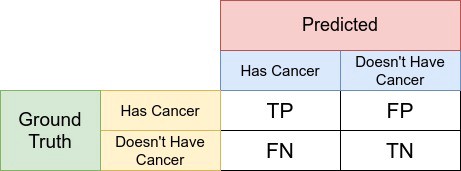
Each cell in the confusion matrix represents an evaluation factor. Let’s understand these factors one by one:
- True Positive(TP) signifies how many positive class samples your model predicted correctly.
- True Negative(TN) signifies how many negative class samples your model predicted correctly.
- False Positive(FP) signifies how many negative class samples your model predicted incorrectly. This factor represents Type-I error in statistical nomenclature. This error positioning in the confusion matrix depends on the choice of the null hypothesis.
- False Negative(FN) signifies how many positive class samples your model predicted incorrectly. This factor represents Type-II error in statistical nomenclature. This error positioning in the confusion matrix also depends on the choice of the null hypothesis.
We can calculate the cell values using the code below:
def find_TP(y, y_hat):
   # counts the number of true positives (y = 1, y_hat = 1)
   return sum((y == 1) & (y_hat == 1))
def find_FN(y, y_hat):
   # counts the number of false negatives (y = 1, y_hat = 0) Type-II error
   return sum((y == 1) & (y_hat == 0))
def find_FP(y, y_hat):
   # counts the number of false positives (y = 0, y_hat = 1) Type-I error
   return sum((y == 0) & (y_hat == 1))
def find_TN(y, y_hat):
   # counts the number of true negatives (y = 0, y_hat = 0)
   return sum((y == 0) & (y_hat == 0))
We’ll look at the Confusion Matrix in two different states using two sets of hyper-parameters in the Logistic Regression Classifier.
from sklearn.linear_model import LogisticRegression
clf_1 = LogisticRegression(C=1.0, class_weight={0:100,1:0.2}, dual=False, fit_intercept=True,
                  intercept_scaling=1, l1_ratio=None, max_iter=100,
                  multi_class='auto', n_jobs=None, penalty='l2',
                  random_state=None, solver='lbfgs', tol=0.0001,       verbose=0,
                  warm_start=False)
clf_2 = LogisticRegression(C=1.0, class_weight={0:0.001,1:900}, dual=False, fit_intercept=True,
                  intercept_scaling=1, l1_ratio=None, max_iter=100,
                  multi_class='auto', n_jobs=None, penalty='l2',
                  random_state=None, solver='lbfgs', tol=0.0001, verbose=0,
                  warm_start=False)
Precision
Precision is the ratio of true positives and total positives predicted:

0<P<1
The precision metric focuses on Type-I errors(FP). A Type-I error occurs when we reject a true null Hypothesis(H⁰). So, in this case, Type-I error is incorrectly labeling cancer patients as non-cancerous.
A precision score towards 1 will signify that your model didn’t miss any true positives, and is able to classify well between correct and incorrect labeling of cancer patients. What it cannot measure is the existence of Type-II error, which is false negatives – cases when a non-cancerous patient is identified as cancerous.
A low precision score (<0.5) means your classifier has a high number of false positives which can be an outcome of imbalanced class or untuned model hyperparameters. In an imbalanced class problem, you have to prepare your data beforehand with over/under-sampling or focal loss in order to curb FP/FN.
For Set-I hyperparameters:
TP = find_TP(y, y_hat)
FN = find_FN(y, y_hat)
FP = find_FP(y, y_hat)
TN = find_TN(y, y_hat)
print('TP:',TP)
print('FN:',FN)
print('FP:',FP)
print('TN:',TN)
precision = TP/(TP+FP)
print('Precision:',precision)
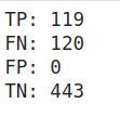

Output for the above code snippet
As you would have guessed by looking at the confusion matrix values, that FP’s are 0, so the condition is perfect for a 100% precise model on a given hyperparameter setting. In this setting, no type-I error is reported, so the model has done a great job to curb incorrectly labeling cancer patients as non-cancerous.
For set-II hyperparameters:
TP = find_TP(y, y_hat)
FN = find_FN(y, y_hat)
FP = find_FP(y, y_hat)
TN = find_TN(y, y_hat)
print('TP:',TP)
print('FN:',FN)
print('FP:',FP)
print('TN:',TN)
precision = TP/(TP+FP)
print('Precision:',precision)
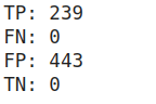

Output for the above code snippet
Since only type-I error remains in this setting, the precision rate goes down despite the fact that type-II error is 0.
We can deduce from our example that only precision cannot tell you about your model performance on various grounds.
Recall/Sensitivity/Hit-Rate
A Recall is essentially the ratio of true positives to all the positives in ground truth.

0<R<1
The recall metric focuses on type-II errors(FN). A type-II error occurs when we accept a false null hypothesis(H⁰). So, in this case, type-II error is incorrectly labeling non-cancerous patients as cancerous.
Recall towards 1 will signify that your model didn’t miss any true positives, and is able to classify well between correctly and incorrectly labeling of cancer patients.
What it cannot measure is the existence of type-I error which is false positives i.e the cases when a cancerous patient is identified as non-cancerous.
A low recall score (<0.5) means your classifier has a high number of false negatives which can be an outcome of imbalanced class or untuned model hyperparameters. In an imbalanced class problem, you have to prepare your data beforehand with over/under-sampling or focal loss in order to curb FP/FN.
For set-I hyperparameters:
TP = find_TP(y, y_hat)
FN = find_FN(y, y_hat)
FP = find_FP(y, y_hat)
TN = find_TN(y, y_hat)
print('TP:',TP)
print('FN:',FN)
print('FP:',FP)
print('TN:',TN)
recall = recall_score(y, y_hat)
print('Recall: %f' % recall)


Output for the above code snippet
From the above confusion matrix values, there is 0 possibility of type-I errors and an abundance of type-II errors. That’s the reason behind the low recall score. It only focuses on type-II errors.
For set-II hyperparameters:
TP = find_TP(y, y_hat)
FN = find_FN(y, y_hat)
FP = find_FP(y, y_hat)
TN = find_TN(y, y_hat)
print('TP:',TP)
print('FN:',FN)
print('FP:',FP)
print('TN:',TN)
recall = recall_score(y, y_hat)
print('Recall: %f' % recall)


Output for the above code snippet
The only error that’s persistent in this set is type-I errors and no type-II errors are reported. This means that this model has done a great job to curb incorrectly labeling non-cancerous patients as cancerous.
The major highlight of the above two metrics is that both can only be used in specific scenarios since both of them identify only one set of errors.
Precision-Recall tradeoff
To improve your model, you can either improve precision or recall – but not both! If you try to reduce cases of non-cancerous patients being labeled as cancerous (FN/type-II), no direct effect will take place on cancerous patients being labeled as non-cancerous.
Here’s a plot depicting the same tradeoff:
from sklearn.metrics import plot_precision_recall_curve
disp = plot_precision_recall_curve(clf, X, y)
disp.ax_.set_title('2-class Precision-Recall curve: '
                  'AP={0:0.2f}'.format(precision))

This tradeoff highly impacts real-world scenarios, so we can deduce that precision and recall alone aren’t very good metrics to rely on and work with. That’s the reason you see many corporate reports and online competitions urge the submission metric to be a combination of precision and recall.
F1-score
The F1-score metric uses a combination of precision and recall. In fact, the F1 score is the harmonic mean of the two. The formula of the two essentially is:
Now, a high F1 score symbolizes a high precision as well as high recall. It presents a good balance between precision and recall and gives good results on imbalanced classification problems.
A low F1 score tells you (almost) nothing — it only tells you about performance at a threshold. Low recall means we didn’t try to do well on very much of the entire test set. Low precision means that, among the cases we identified as positive cases, we didn’t get many of them right.
But low F1 doesn’t say which cases. High F1 means we likely have high precision and recall on a large portion of the decision (which is informative). With low F1, it’s unclear what the problem is (low precision or low recall?), and whether the model suffers from type-I or type-II error.
So, is F1 just a gimmick? Not really, it’s widely used, and considered a fine metric to converge onto a decision, but not without some tweaks. Using FPR (false positive rates) along with F1 will help curb type-I errors, and you’ll get an idea about the villain behind your low F1 score.
For set-I hyperparameters:
# F1_score = 2*Precision*Recall/Precision+Recall
f1_score = 2*((precision*recall)/(precision+recall))
print('F1 score: %f' % f1_score)
If you recall our scores in set-I parameters were, P=1 and R=0.49. Thus, by employing both of the metrics we get a score of 0.66 which doesn’t give you information about what type of error is significant, but is still useful in deducing the performance of the model.
For set-II hyperparameters:
# F1_score = 2*Precision*Recall/Precision+Recall
f1_score = 2*((precision*recall)/(precision+recall))
print('F1 score: %f' % f1_score)

For set-II, parameters were, P=0.35 and R=1. So again, the F1 score sort of sums up the break between P and R. Still, low F1 doesn’t tell you which error is happening.
F1 is no doubt one of the most popular metrics to judge model performance. It’s actually a subset of wider metrics known as the F-scores.
Putting in beta=1 will fetch you the F1 score.
AUROC (Area under Receiver operating characteristics curve)
Better known as AUC-ROC score/curves. It makes use of true positive rates(TPR) and false positive rates(FPR).

- Intuitively TPR/recall corresponds to the proportion of positive data points that are correctly considered as positive, with respect to all positive data points. In other words, the higher the TPR, the fewer positive data points we will miss.
- Intuitively FPR/fallout corresponds to the proportion of negative data points that are mistakenly considered as positive, with respect to all negative data points. In other words, the higher the FPR, the more negative data points we will misclassify.
To combine the FPR and the TPR into a single metric, we first compute the two former metrics with many different thresholds for the logistic regression, then plot them on a single graph. The resulting curve is called the ROC curve, and the metric we consider is the area under this curve, which we call AUROC.
from sklearn.metrics import roc_curve
from sklearn.metrics import roc_auc_score
from matplotlib import pyplot
ns_probs = [0 for _ in range(len(y))]
# predict probabilities
lr_probs = clf_1.predict_proba(X)
# keep probabilities for the positive outcome only
lr_probs = lr_probs[:, 1]
# calculate scores
ns_auc = roc_auc_score(y, ns_probs)
lr_auc = roc_auc_score(y, lr_probs)
# summarize scores
print('No Skill: ROC AUC=%.3f' % (ns_auc))
print('Logistic: ROC AUC=%.3f' % (lr_auc))
# calculate roc curves
ns_fpr, ns_tpr, _ = roc_curve(y, ns_probs)
lr_fpr, lr_tpr, _ = roc_curve(y, lr_probs)
# plot the roc curve for the model
pyplot.plot(ns_fpr, ns_tpr, linestyle='--', label='No Skill')
pyplot.plot(lr_fpr, lr_tpr, marker='.', label='Logistic')
pyplot.xlabel('False Positive Rate')
pyplot.ylabel('True Positive Rate')
pyplot.legend()
pyplot.show()

Logistic: ROC AUC=0.996
A no-skill classifier is one that can’t discriminate between the classes, and would predict a random class or a constant class in all cases. The no-skill line changes based on the distribution of the positive to negative classes. It’s a horizontal line with the value of the ratio of positive cases in the dataset. For a balanced dataset, it’s 0.5.
The area equals the probability that a randomly chosen positive example ranks above (is deemed to have a higher probability of being positive than negative) a randomly chosen negative example.
So, high ROC simply means that the probability of a randomly chosen positive example is indeed positive. High ROC also means your algorithm does a good job at ranking test data, with most negative cases at one end of a scale and positive cases at the other.