Numerical Data or Quantitative Data
Numerical data or quantitative data consist of numbers. Numeric data points will have mathematical significance to each other or to the labels (column header) like price, distance, area, blood pressure, height, weight, length, salary, some type of count or a measurement represented by a number.
Some algorithms even have assumptions about how data should be in order for them to work well.
Upon numeric data arithmetic operation like average, multiplication makes sense, you can not take out an average of a column containing color categories like red, green, blue, purple, pink, violet.
Numerical data can further be broken down into discrete & continuous data.
Discrete & Continuous Data
Discrete data is counted & continuous data is measured. Upon rolling a dice, we get discrete value like 1, 2, 3, 4, 5 or 6. And upon counting the number of students in a class, we get 12, 20, 25 etc. There is never half a dice roll or quarter of a boy 🙂
Discrete data is counted, breaking the count in smaller intervals will not make sense. Like number of students in a class.
Continuous data is measured over a scale, the scale can be finite or infinite. Continuous data can be broken into smaller and smaller measurement based on the precision of measurement. For example, measuring units of time can be second, millisecond, microsecond, nanosecond, picosecond.
Continuous data is measured over a scale, breaking the measurement in smaller and smaller intervals will also make sense in continuous data.
Remember, if you use counting to find the value, then it is a discrete data. It can not be broken into smaller & smaller fraction or decimal. However, if you use a scale to measure the value then it is continuous data like height, weight, length etc.
Categorical Data or Qualitative Data
Categorical data is a description or a measurement that doesn’t have a numeric meaning like race, gender (male, female), color (red, blue, green), college attended, disease status etc. However, remember that at times we encode categorical data as numeric in machine learning.
Not all integer data is numeric like postal codes (560034). Postal codes should be considered categorical.
How to identify categorical from Numeric data?
Try calculating mathematics operation such as average on the data. Average of birth date or postal code doesn’t make sense, hence consider them as categorical.
Categorical data can further be broken into Ordinal & Nominal data

Levels of measurement: Theory of Levels of measurement was introduced by American psychologist Stanley Smith Stevens in 1946. According to him, there are four measuring scales which are Nominal, Ordinal, Interval and Ratio.
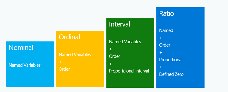
Nominal Scale
It doesn’t have any numerical significance or order. It is a categorization or description of a label. Like gender (male, female), type of living accommodations (house, apartment, villa), religious types (Muslim, Hindu, Christian, Buddhist, Jewish), color(red, blue. green). Here red, blue, green are just colors without any specific order as considering red prior to green.
Nominal variable having only two possible value is called a dichotomous variable. (e.g., age: under 65/65 and over) or an attribute (e.g., gender: male/female)
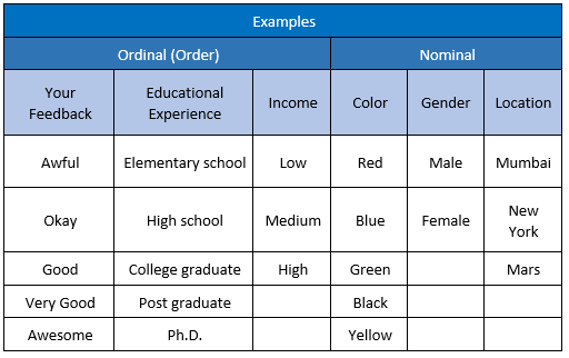
Ordinal Scale
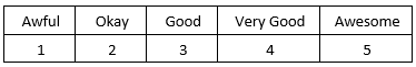
Here, the order of the values have a significance, like in a feedback system lower to higher value categorization will be Awful, Okay, Good, Very Good, Awesome. From ordinal, you get “order”.
Point to note is that here you can not measure the feedback difference (degree of difference) between awful & awesome. However, we understand that awful is dis-satisfactory & awesome considered delightful.
Examples: level of agreement (yes, maybe, no), time of day (dawn, morning, noon, afternoon, dusk, night).
Ordinal allows rank order to sort the data but it doesn’t have a relative degree of difference between the values.
In simple words, if you see a set of data values like Awful, Okay, Good, Very Good, Awesome or yes, maybe, no. Your brain will automatically find a order thinking awful comes before okay. This type of data where order is present by default is ordinal data.
Interval & Ratio scale
In Interval scale or interval variable we know exact different between the measurement of values. Like in between the boiling & freezing point there are 100 intervals. The difference between 20–10 degree Celsius is exactly same as that between 90–80 degree Celsius. Other examples are Fahrenheit temperature & IQ.
Interval scale doesn’t have absolute zero. Values can be negative like in Celsius absolute zero temperature is -273 degree Celsius.
In interval scale values can be added, subtracted, counted but can not be multiplied or divided. Interval scale will not give correct ratios.
Understand with an example: Suppose you are inside a warm room (20 degree Celsius) while it is cold outside (10 degree Celsius).
As per the ratio, temperature inside the room is twice that of outside however that is wrong as per thermodynamics. As per Thermodynamics molecule at 0 Kelvin(-273) will have no heat or energy to vibrate.
Equivalent temperature of 10 Celsius in kelvin scale is = 283.15 Kelvin & twice of that temperature is 2*283.15 = 566.3 Kelvin(293.15 Celsius)
According to thermodynamics twice the temperature of 10 C is 293.15 C not 20 C… mind blowing right 🙂
Kelvin is Ratio variable while Celsius is Interval variable
Interval scale gives us clear understanding of differences in temperature, inside the room is 10 degree more than outside however it can not be used to calculate ratios. Another interval variable is pH, pH=2 is not twice acidic as pH=4.
Ratio scale or variables
Ratio scale have a clear definition of 0.0 (Absolute zero or zero). Variables like height, time (m sec, hours), length(cm, kilometer), volume(cc) & weight are all ratio variables. Weight, height can be calculated between zero and maximum however there is nothing like -5 feet height.
Sample Theory
A Population stands for all the observations that exists for that variable, like height of all men in existence, past & future combined for a research. Such a dataset is hypothetical & does not exist at least till now.
Sample is a subset of this population that is used for the research like height of all men in India. There are ways to collect samples like random sampling, stratified sampling, cluster sampling & its study is called sample theory.
In Random sampling any observation from the population can be selected in the sample, probability of selection is same for all observations.
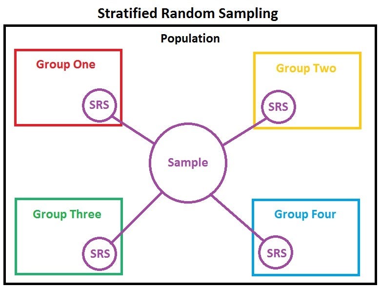
In stratified sampling entire population is divided into smaller groups called strata/ stratum based on common data characteristics like similar age, gender, nationality or education. Each element in the population is only assigned to one strata. Observations are mostly selected randomly from each strata. Stratified sampling reduces sampling error as sample contain members from all stratas giving sample same characteristic as the population.
Mean
Mean is the average of a set numbers x1, x2, …, xn, it can be obtained by simply adding all of them and dividing by total number of observations (x1+ x2, … + xn)/n. Mean of a sample is called sample mean & for a population as population mean. Mean is effected if there are extreme values in the dataset.
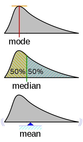
Median
Median is the value dividing the sample in two equal halves, where one half of values lie above the median while other half lies below it. When observations are arranged in an increasing order( lowest value to the highest value) median is the “middle value”, like in the data set {1, 3, 3, 6, 7, 8, 9}, the median is 6. Median is (N+1)/2th term when numbers are odd.
When number of observations are even like 1,2,3,4,5,6,8,9 it is (4+5)/2 = 4.5 i.e. [(N/2th) + (N+1/2th)]/2… average of two middle values.
Median is the value dividing the sample in two equal halves, where one half of values lie above the median while other half lies below it.
Median value is the quoted figure when dealing with property prices as mean of property prices will be affected by few expensive properties not representing general market.
Mode
Mode of a set of data values is the value that appears most often. Like manufacturing most popular shoes, because manufacturing all shoes in equal number will cause oversupply of non-popular shoes. It is possible for dataset to have more than one mode. If there are two data values that occur most frequently, we say that the set of data values is bimodal. Also, if there is no value that occurs most frequently then there is no mode.
Mean, median & mode are collectively are known as measure of central tendency as they infers where the data is clustered or centered.
Dispersion (also called variability, scatter, or spread) quantify the spread of data, like how dispersed data is from the mean. Measure of dispersion are variance, standard deviation, and interquartile range. Range is the difference between the largest & smallest data observation.
Variance
Variance measures how far each number in the set is from the mean. variance is calculated by taking the differences of each number in the set and mean, squaring the difference and dividing the sum of squares by the number of values in the set. Putting simply … variance is the average of the squared differences from the Mean.
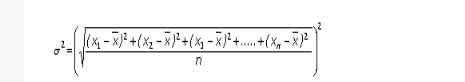
Variance is the square of the standard deviation
Unlike range, variance take in consideration all data points in a data set to produce the spread.
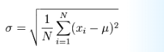
Standard Deviation
Standard deviation σ (the greek letter sigma) is a measure of the spread of numbers.
Standard Deviation is the square root of Variance … its not me, that’s how stat geeks define it !!
Significance: By marking all values that are within one Standard deviation of the mean, you can know what is a normal value, and what is extra small or extra large value. For example
Histogram
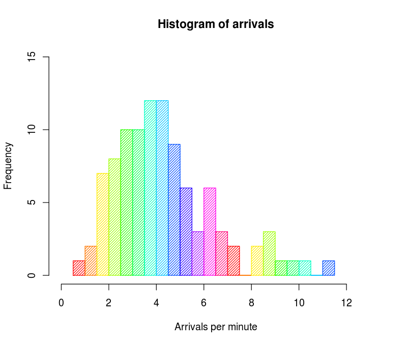
Histogram is a frequency distribution that shows how often each value in a set occurs, it is a quick way to get information about a sample.
First step to create a histogram is by creating a “bin” or “bucket”. Bin stands for dividing the entire series of values into intervals and then count how many values fall into each.
Highest peak or the value that repeats the most is mode
Bins are mostly non-overlapping intervals generally of equal size. Height of the rectangle over a bin represent frequency or number of observations falling in that bin.
Plotting a histogram will show whether data distribution is normally distributed or skewed.
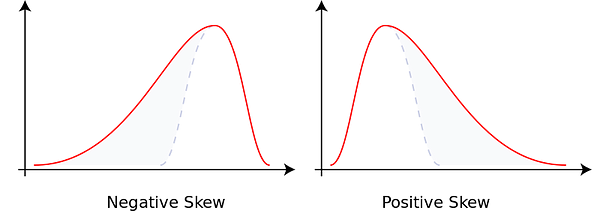
Skewness
Skewness is the asymmetry in a distribution, curve appears to be distorted either to left or right.
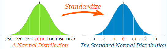
Normal Distribution
When data tends to be around a central value making a bell curve without skewness, it is called as normal distribution or Gaussian distribution.

Data that follow a normal distribution- particles experiencing diffusion, blood pressure, IQ, error in measurement or measure of liquid filled in coke bottle.
Normal distribution has overlapping mean, mode, median. Standard deviation σ (the greek letter sigma) is a measure of how spread out numbers are.
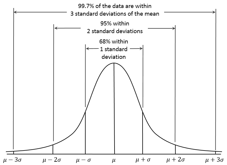
Generally 68 % of values are within 1 standard deviation, 95% between 2 standard deviation, 99.7% within 3 standard deviations. “Standard Score”, “sigma” or “z-score” is the number of standard deviation from mean. Like if data points z score is 2 then it is two standard deviations far from mean.
Non-normal data can be transformed to normal by applying log, square root or similar transformations. Some machine learning algorithms like LDA , gaussian naive bayes assumes underlying data to be normal.
Correlation
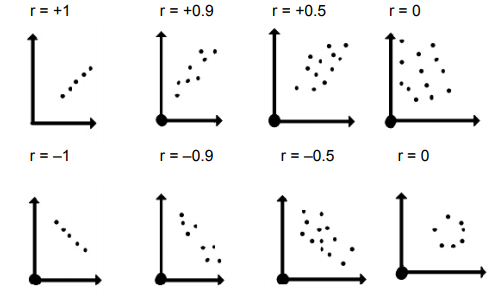
Correlation is when the change in one item may result in the change in another item, its value lies between -1 and 1. Significance of correlation lies in fact that it can be used to predict one variable from another.
Correlation is positive if both variables values increase together & negative when one value decreases while other increases. For example, Ice-cream sales increases with increase in temperature, two stocks rising together, sales increasing with new marketing strategy in place.
What is Causal Relation: A causal relation between two events imply that first event causes other. First event is called as cause and other event is the effect. Two event having causal relation will be correlated but correlated events might not be causal.
Correlation Is Not Causation
Remember just by calculating correlation (Pearson’s Correlation) between two variables it is not provable that one causes other to change.
- Perfect correlation = 1
- No correlation = 0
- Perfect negative correlation = -1
Correlation does not show causal relationship, For example In behavioral science depression and self esteem are significantly correlated however we can not certainly say depression is caused by low self esteem, culprit might be stress, genetics, drugs others.
Note: In correlation
- Association or relationship between correlated variable may just be random.
- First variable might have caused change in other variable.
- Other variable might have effected first variable.
- Variables might be depending on another third variable causing them to vary together…No guarantees anywhere.
Correlation is represented best by a scatter plot
Scatter plot looks different for different values of correlation.
Can anyone answer in the comments below the risk involved while investing in 100 stocks which are all positively correlated?
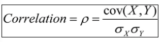
Covariance
Correlation is when the change in one item may result in the change in another item, Covariance is when two item vary together. Its value lies between -∞ and +∞.
Covariance measures linear relation between variables.
Covariance is a measure of correlation, on the contrary, correlation refers to the scaled form of covariance i.e. putting values that are in between -∞ & +∞ (covariance) to -1 &+1 (correlation).
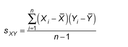
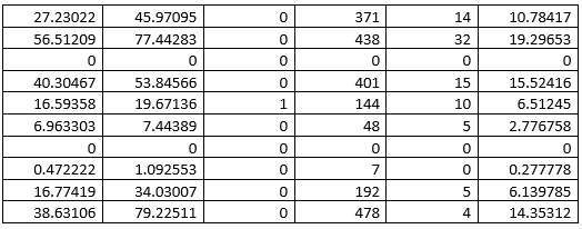
Calculating Covariance & Correlation
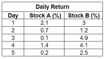
Mean of A = 0.9, mean of B =3.14, σx = 0.8456, σy = 1.4328
Covariance = (2.1–0.9)(3–3.14) +(0.7–0.9)(1.2–3.14)… (0.2–0.9)(2.5–3.14)/(5–1)
Covariance = -0.065
Correlation = -0.0536
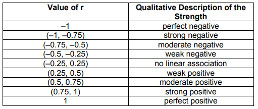
Covariance is negative hence these two stocks move in opposite directions. If one tends to have a higher return then other will not. Also when the value of correlation is close to zero, generally between -0.1 and +0.1, the variables are said to have no linear relationship or a very weak linear relationship
Data is the most important part of data analysis, machine learning or deep learning, hence my efforts will continue to produce all important information, approaches to data science in one place for everyone to learn from.