While data science/machine learning is a complicated sector, as it core, it is very intuitive. Hence, I believe explaining these difficult task with simple examples can better help you understand why these methods/ideas work.

Hence, we will proceed with a simple example.

We build 4 models using Linear Regression, Lasso Regression, Ridge Regression, and Random Forest Regressor for 4 people (remember, simple example). We predicted $1,000, $1,500, $2,000, and $2,500 for user_1, user_2, user_3, and user_4, respectively. The ground truth for user_1, user_2, user_3, and user_4 was $980, $1,943, $1,239, and $2,020, respectively.

How should we evaluate our predictions?

For prediction:
980 + 1943 + 1239 + 2020 = 6182For ground truth:
1000 + 1500 + 2000 + 2500 = 7000# Difference
7000 - 6182 = 818

So, does the difference of $818 tell us anything about our model’s performance?

Well, let’s discuss another example first.

Using another model, the predictions were $1,000, $1,500, $2,000, and $3,318.

For prediction:
1000 + 1500 + 2000 + 3318 = 7818For ground truth:
1000 + 1500 + 2000 + 2500 = 7000# Difference
7000 - 7818 = -818

There are a couple of things to notice:

• Does the sign (negative or positive) make a difference? Is 818 or -818 preferred?
• Even though the absolute difference was the same, the predictions are different. Prediction for the second set of salaries correctly predicted salaries except for one person. Yet, the absolute difference does not show this.

Cool story bro, but how can we better judge performance?

I am glad you asked “bro.”

Mean Absolute Error (MAE)

The Mean Absolute Error measures the average of the absolute difference between each ground truth and the predictions. Whether the predictions is 10 or 6while the ground truth was 8, the absolute difference is 2.

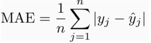
The y^hat is the prediction but again, the order doesn’t matter since we are calculating the absolute contrast.

In our example above, the result would be:

|1000 — 980| = 20
|1500 — 1943| = 443
|2000 — 1239| = 761
|2500 — 2020| = 480# The average of the error summation
(20 + 443 + 761 + 480) / 4 = 426

Now, what does $426 mean? Is my model performing well?

Like the RMSE (which will be explained later), the MAE is an absolute measure of fit. “It can be interpreted as the standard deviation of the unexplained variance, and has the useful property of being in the same units as the response variable.”

Or in layman’s term, we should expect our prediction to be off by 426 (on average) from the ground truth.

Notes:

• Evaluating how well our model is more subjective than objective. Using the example above, the 426 might seem our model is performing great if people’s salary ranged from $100 to $100,000,000. But if the range is from $1,000 to $2,500, 426 indicates our model is underperforming.
• For some problems, you might be assigned an MAE threshold. Hence, this could help you gauge performance. If not, the dependent variable can help us assess our performance. As explained above, the datum’s dependent variable ranges from $1,000 to $2,500. An MAE of $426 conveys that we should expect, on average, a difference of $426, which is pretty high given the range of our dependent variable.

Root Mean Squared Error (RMSE)

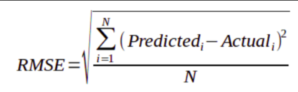
The Root Mean Squared Error measures the square root of the average of the squared difference between the predictions and the ground truth.

(1000 — 980)^2 = 400
(1500 — 1943)^2 = 196249
(2000 — 1239)^2 = 579121
(2500 — 2020)^2 = 230400# The average of the square error summation
(400 + 196249 + 579121 + 230400) / 4 = 251543# Square root of the square error summation
Square root of $251,543 is ~$502

Notice that the RMSE is larger than the MAE. Since the RMSE is squaring the difference between the predictions and the ground truth, any significant difference is made more substantial when it is being squared. RMSE is more sensitive to outliers.

Hence, if the outliers are undesirable, the RMSE better evaluates how well your model is performing. Also, like the MAE, the smaller the result, the better your model is performing.

Notes:

1. The MAE/RMSE are in the same units as the dependent variable. Hence, MAE/RMSE must be compared with the dependent variable.
2. More mathematically, if you would like to use the RMSE as a cost function (or MSE), it is “smoothly differentiable.” Of course, you do not need to understand the implications of the MAE or RMSE as a cost function. Just know, it makes calculating gradient descent for easily. If you would like to know more, you should read this Quora post.

R-Squared

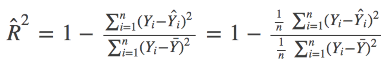
If you like to understand how well the independent variables “explain” the variance in your model, the R-Squared formula can be powerful.

As you’ll notice in the image, the formula appears complicated (it is not!).

To calculate how well our model does in explained the variance of our model, we need to figure the SSR, SSE, and SSTO (the terminology might change depending on how you’re learning the material).

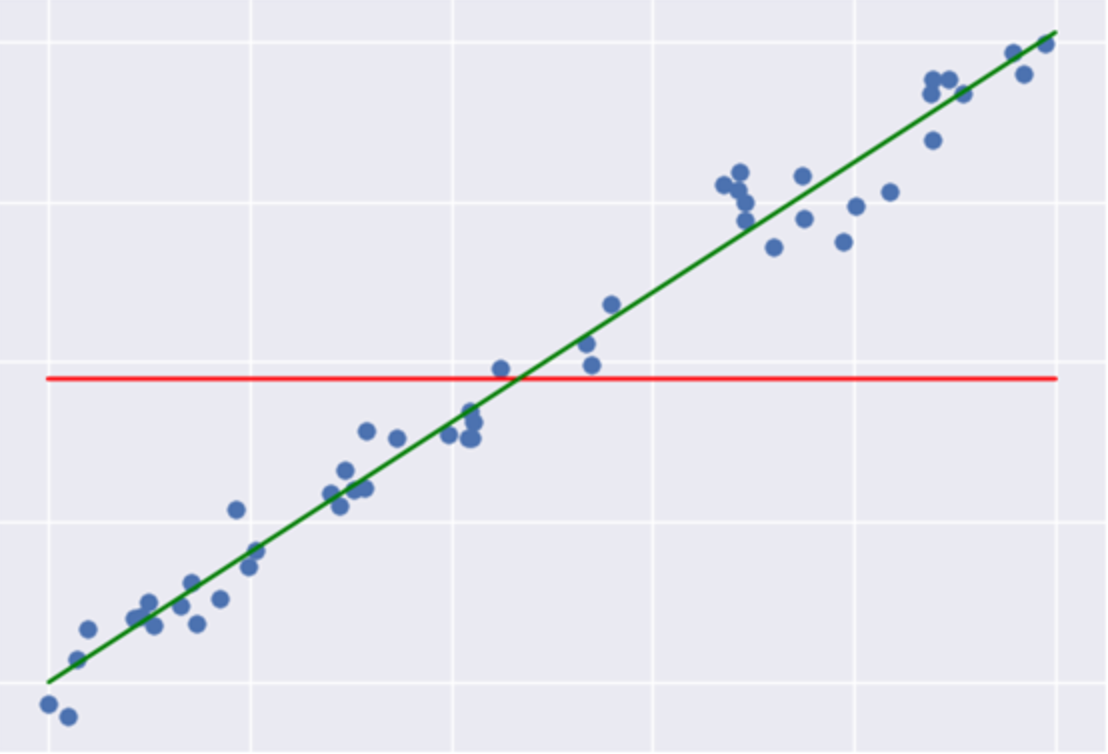
SSR: Regression Sum of Squares quantifies how far the estimated sloped regression line (green line) is from the horizontal (red line). The red line is the average of the ground truth.

SSE: Error sum of squares quantifies how much the data points (blue dots) is from the prediction (green line).

SSTO: Total Sum of Squares quantifies how much the data points (blue dot) is from the horizontal (red line).

SSTO = SSE + SSR

R-Squared = SSR / SSTO

# The total difference minus the error
SSR = SSTO - SSER^Squared = SSR / SSTO# Substitute SSR into the equation
R^Squared = (SSTO - SSE) / SSTO
R^Squared = (SSTO / SSTO) - (SSE / SSTO)
R^Squared = 1 - (SSE / SSTO)

The weaker the variance between our model and the linear model is, the stronger the R^Squared.

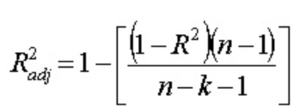
Adjusted R-squared

One of the pitfalls of the R-squared is that it will always improve as we increase the number of variables.

Why? Well, think about it. If your model has an R-Squared of .43, and then you train a more complicated model (with more variables) there are only two things that could happen.

1. The additional variables do not improve the model at all.
2. The additional variables improve the model.

Performance cannot decrease because you are including more variables which will make the model better fit the data!

The Adjusted R-Squared fixes this problem. It adds a penalty to the model. Notice that there are two additional variables in the model.

The n represents the total number of observations. The k represents the total number of variables in your model.

Focus on the equation above. As you increase the number of variables (keeping everything else constant), you are decreasing the denominator. Hence, you are increasing the left side of the equation (inside the brackets). Since we are subtracting by 1, we are lowering the Adjusted R-Squared. Hence, the improvement in the model must be stronger than the penalty for the Adjusted R-Squared to improve as we increase the number of variables.

Notes:

• For the R-Squared and the Adjusted R-Squared, the closer the value to 1, the better performer our model!
• RMSE/MAE is used to evaluate the variance in the errors. Additionally, the value within itself doesn’t tell you much. You must compare different models to reap from the RMSE/MAE.
• However, R-Square/Adjusted R-Squared doesn’t need to be compared between different models. If the R-Squared/Adjusted R-Squared is .10, we can acknowledge that the model is not doing a great job is modeling.