Shapley Values
Let’s Play a Game
When a team of eleven players goes on to win the World Cup, who is the most valuable player? Shapley value is a decomposition algorithm that objectively distributes the final result to a pool of factors. In explaining a machine learning model, Shapley values can be understood as the significance of individual input features’ contribution to the model’s predicted values.
A Quick Example — How does Shapley value work?
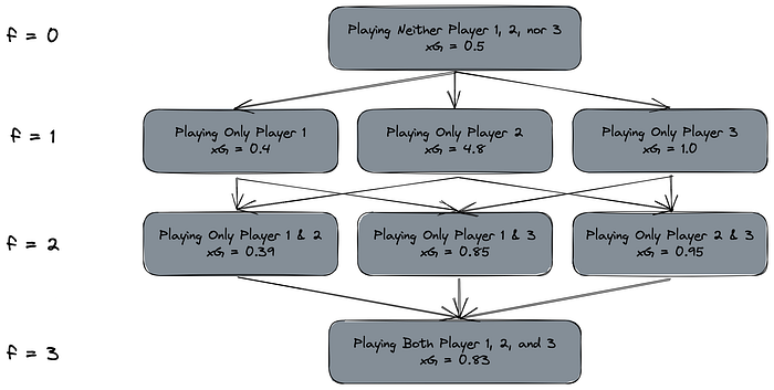
For simplicity’s sake, let’s say we have three attacking players, each with a different expected number of goals. We also know that these three players don’t always work well with each other, which means depending on the combination of the three players, the number of expected goals may be different:

As a baseline, we play none of these three players i.e. number of features f = 0 and the expected number of goals of the team will be 0.5. Each of the arrow that goes down the matrice indicates a possible stepwise increment when including a new feature (or including a player in our case).
Following the idea of stepwise expansion of player set, that means we can compute the marginal change for each of the arrow. For example, when we move from playing none of the players (indicated with the empty set symbol ∅) to playing player 1 only, the marginal change is:

To obtain the overall contribution of Player 1 among all three players, we would have to repeat the same calculation for every scenario where a marginal contribution for Player 1 is possible:

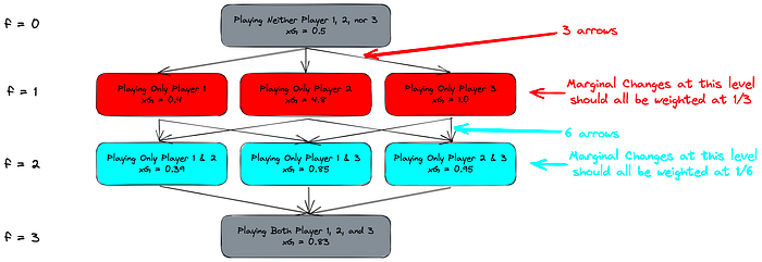
With all the marginal changes, we then calculate the weights for them using the following formula:

Or, to put it even simpler: it is just the reciprocal of the number of all edges pointing into the same row. That means:

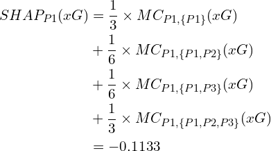
With this, we can now calculate the SHAP value of Player 1 for the expected goals:

Repeating for the other two players and we will have:
- SHAP of Player 1 = -0.1133
- SHAP of Player 2 = -0.0233
- SHAP of Player 3 = +0.4666
If I were the head coach, I would have only played Player 3 in this case.
