Please follow the steps to complete your e-attendance

• Click this link

Primary Requirements

• Some programming experience (e.g. C, C++, Java, QBasic (!) etc. )
• At least high school level math skills will be required.
• Passion to learn

IDE Requirements

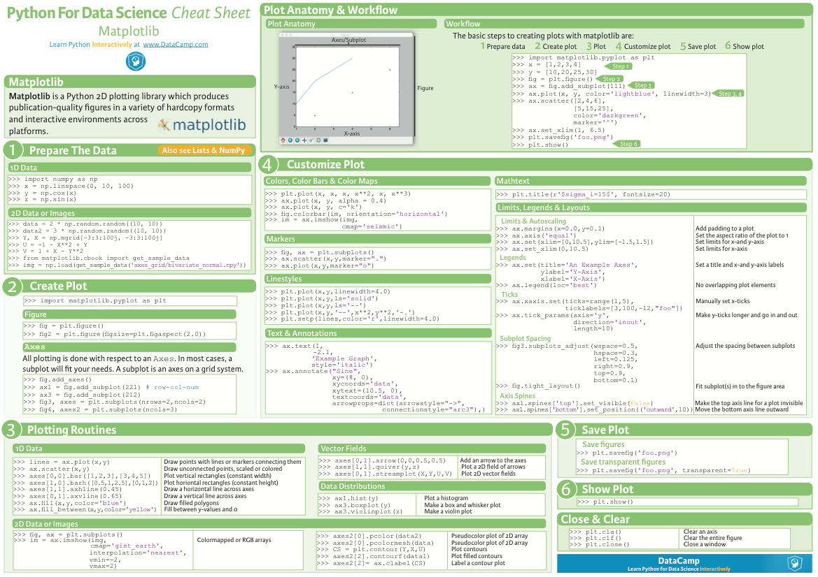
• Most popular IDE for Data Science is Anaconda. You can download and install from here. Make sure your download Python 3.7 distribution. 

F.A.Q

» I don’t have the admin permission to install any software (Don’t worry !)

•  Google Colab [if you already have Google Account ]
• Azure Notebook [if you already have Microsoft Account]
• Both are Free ! to use

»  Is there anyway I can do Machine Learning Analytics with Less Code or No Code?

Yes ! We can. 

»  Really ? How to do that?

Step 1 : Please go to this site https://studio.azureml.net/

Step 2 : Use any Microsoft Account(youremail@hotmail.com / outlook.com) to Register and Login

Module 1: Introduction to Data Science

Data Scientist has been ranked the number one job on Glassdoor and the average salary of a data scientist is over $120,000 in the United States according to Indeed! Data Science is a rewarding career that allows you to solve some of the world’s most interesting problems! In this Module we will experience an intro of Data Science and it’s different arena in simple way. 

Module 2: No-Code Machine Learning

This module introduces the Designer tool, a drag and drop interface for creating machine learning models without writing any code. You will learn how to create a training pipeline that encapsulates data preparation and model training, and then convert that training pipeline to an inference pipeline that can be used to predict values from new data, before finally deploying the inference pipeline as a service for client applications to consume.

Hands-on : Design a Machine Learning Model using ML Studio

Module 3: Python – A Quick Review

In this module, you will get a quick review on Python Language. We will not going in depth but we will try to discuss some important components of Python Language. Please note, this is not meant to be a comprehensive overview of Python or programming in general 

Hands-on : Environment Setup and  Jupyter Notebook Intro. 

Hands-on : Python Code Along

Hands-on : Python Review Exercise

Presentation File:

Machine Learning – Introduction

Related Materials:

• Data Concept
  • To know more about Data Concept you can click [this] link.
• ML Performance Metrics:
  • For Supervised Machine Learning
• AzureML End-to-End Lecture Series 
  • Doing Machine Learning with Azure ML (3-day course)

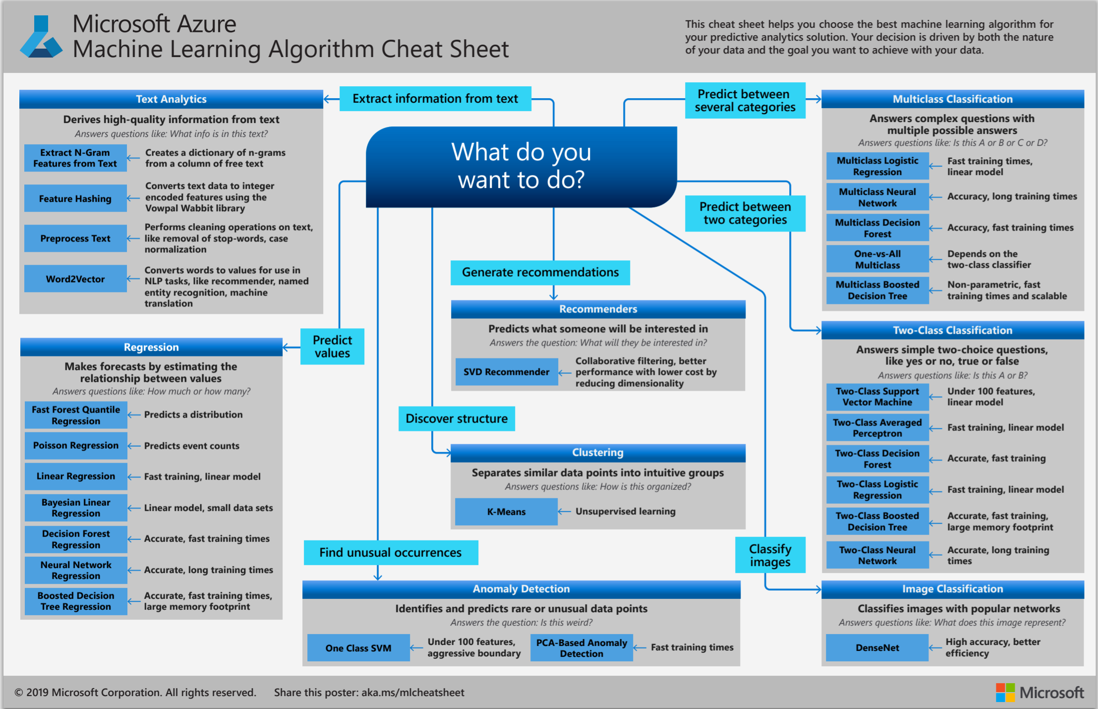
Azure ML Cheat Sheet

Algorithm Summary

Source: http://machinelearningmastery.com/a-tour-of-machine-learning-algorithms/

 

 

Python Packages Cheat Sheet

Source: http://datasciencefree.com/python.pdf

 

 

[NumPy]

Source: https://s3.amazonaws.com/assets.datacamp.com/blog_assets/Numpy_Python_Cheat_Sheet.pdf

 

[Pandas]

Source: http://datacamp-community-prod.s3.amazonaws.com/dbed353d-2757-4617-8206-8767ab379ab3

 

 

[Matplotlib]

Source: https://s3.amazonaws.com/assets.datacamp.com/blog_assets/Python_Matplotlib_Cheat_Sheet.pdf

 

 

[Scikit Learn]

Source: https://s3.amazonaws.com/assets.datacamp.com/blog_assets/Scikit_Learn_Cheat_Sheet_Python.pdf

 

Automobile Price Prediction  

The Problem

This data set consists of three types of entities: (a) the specification of an auto in terms of various characteristics, (b) its assigned insurance risk rating, (c) its normalized losses in use as compared to other cars. The second rating corresponds to the degree to which the auto is more risky than its price indicates. Cars are initially assigned a risk factor symbol associated with its price. Then, if it is more risky (or less), this symbol is adjusted by moving it up (or down) the scale. Actuarians call this process “symboling”. A value of +3 indicates that the auto is risky, -3 that it is probably pretty safe.

The third factor is the relative average loss payment per insured vehicle year. This value is normalized for all autos within a particular size classification (two-door small, station wagons, sports/speciality, etc…), and represents the average loss per car per year.

Note: Several of the attributes in the database could be used as a “class” attribute.

Please bring it on whatever inferences you can get it and Make a Price Prediction Model. 

The Data

This dataset consist of data From 1985 Ward’s Automotive Yearbook. Here are the sources

Sources:

1) 1985 Model Import Car and Truck Specifications, 1985 Ward’s Automotive Yearbook.
2) Personal Auto Manuals, Insurance Services Office, 160 Water Street, New York, NY 10038
3) Insurance Collision Report, Insurance Institute for Highway Safety, Watergate 600, Washington, DC 20037

Datasets is available Azure ML Studio Saved Datasets > Samples > Automobile Price Data (Raw)

Walmart Store Sales Forecasting  

The Problem

One challenge of modeling retail data is the need to make decisions based on limited history. If Christmas comes but once a year, so does the chance to see how strategic decisions impacted the bottom line.

You are provided with historical sales data for 45 Walmart stores located in different regions. Each store contains a number of departments, and you are tasked with predicting the department-wide sales for each store.

In addition, Walmart runs several promotional markdown events throughout the year. These markdowns precede prominent holidays, the four largest of which are the Super Bowl, Labor Day, Thanksgiving, and Christmas. The weeks including these holidays are weighted five times higher in the evaluation than non-holiday weeks. Part of the challenge presented by this competition is modeling the effects of markdowns on these holiday weeks in the absence of complete/ideal historical data.

The Data

stores.csv

This file contains anonymized information about the 45 stores, indicating the type and size of store.

train.csv

This is the historical training data, which covers to 2010-02-05 to 2012-11-01. Within this file you will find the following fields:

• Store – the store number
• Dept – the department number
• Date – the week
• Weekly_Sales –  sales for the given department in the given store
• IsHoliday – whether the week is a special holiday week

test.csv

This file is identical to train.csv, except we have withheld the weekly sales. You must predict the sales for each triplet of store, department, and date in this file.

features.csv

This file contains additional data related to the store, department, and regional activity for the given dates. It contains the following fields:

• Store – the store number
• Date – the week
• Temperature – average temperature in the region
• Fuel_Price – cost of fuel in the region
• MarkDown1-5 – anonymized data related to promotional markdowns that Walmart is running. MarkDown data is only available after Nov 2011, and is not available for all stores all the time. Any missing value is marked with an NA.
• CPI – the consumer price index
• Unemployment – the unemployment rate
• IsHoliday – whether the week is a special holiday week

Here are the data for download:

• stores
• train
• features
• test

Bike Sharing Demand
Forecast use of a city bikeshare system

The Problem

Bike sharing systems are new generation of traditional bike rentals where whole process from membership, rental and return back has become automatic. Through these systems, user is able to easily rent a bike from a particular position and return back at another position. Currently, there are about over 500 bike-sharing programs around the world which is composed of over 500 thousands bicycles. Today, there exists great interest in these systems due to their important role in traffic, environmental and health issues.

Apart from interesting real world applications of bike sharing systems, the characteristics of data being generated by these systems make them attractive for the research. Opposed to other transport services such as bus or subway, the duration of travel, departure and arrival position is explicitly recorded in these systems. This feature turns bike sharing system into a virtual sensor network that can be used for sensing mobility in the city. Hence, it is expected that most of important events in the city could be detected via monitoring these data.

Data Fields

datetime – hourly date + timestamp  
season –  1 = spring, 2 = summer, 3 = fall, 4 = winter 
holiday – whether the day is considered a holiday
workingday – whether the day is neither a weekend nor holiday
weather – 1: Clear, Few clouds, Partly cloudy, Partly cloudy
2: Mist + Cloudy, Mist + Broken clouds, Mist + Few clouds, Mist
3: Light Snow, Light Rain + Thunderstorm + Scattered clouds, Light Rain + Scattered clouds
4: Heavy Rain + Ice Pallets + Thunderstorm + Mist, Snow + Fog 
temp – temperature in Celsius
atemp – “feels like” temperature in Celsius
humidity – relative humidity
windspeed – wind speed
casual – number of non-registered user rentals initiated
registered – number of registered user rentals initiated
count – number of total rentals

Datasets 

Datasets is available Azure ML Studio Saved Datasets > Samples > Bike Rental UCI Dataset

Heart Diseases Prediction

The Problem

The term “heart disease” is often used interchangeably with the term “cardiovascular disease”. Cardiovascular disease generally refers to conditions that involve narrowed or blocked blood vessels that can lead to a heart attack, chest pain (angina) or stroke. Other heart conditions, such as those that affect your heart’s muscle, valves or rhythm, also are considered forms of heart disease.

This makes heart disease a major concern to be dealt with. But it is difficult to identify heart disease because of several contributory risk factors such as diabetes, high blood pressure, high cholesterol, abnormal pulse rate, and many other factors. Due to such constraints, scientists have turned towards modern approaches like Data Science and Machine Learning for predicting the disease.

The Data

In this practicec, we will be applying Machine Learning approaches (and eventually comparing them) for classifying whether a person is suffering from heart disease or not, using one of the most used dataset — Cleveland Heart Disease dataset from the UCI Repository.

Data Source URL : http://archive.ics.uci.edu/ml/machine-learning-databases/heart-disease/processed.cleveland.data

Solution

There are two ways we can do this; either we can solve this with Azure ML Designer (No Code) way or We can do this using python notebook. 

• Let’s do this using Azure ML Designer (Azure ML Studio -Classic)
• If you’re Python savvy you can follow [this] link for get your ipynb files and to read the blog about this problem scope you can visit this [link]

Hints: 

• Edit Metadata info and put new column name : age,sex,chestpaintype,resting_blood_pressure,serum_cholestrol,fasting_blood_sugar,resting_ecg,max_heart_rate,exercise_induced_angina,st_depression_induced_by_exercise,slope_of_peak_exercise,number_of_major_vessel,thal,heart_disease_diag
• Edit Metadata info and Change Data type to Integer for following Columns:  heart_disease_diag,age,sex
• Edit Metadata info and make it categorical for following Columns: sex,chestpaintype,exercise_induced_angina,number_of_major_vessel,slope_of_peak_exercise,fasting_blood_sugar,thal,resting_ecg
• Clean Missing Value
• Apply SQL Transformation

SELECT *, 
CASE 
WHEN heart_disease_diag < 1 THEN 0
ELSE 1 
END AS HeartDiseaseCat 
FROM t1; 

Dataset Download

heart_data

One Drive

• https://rb.gy/t74leq (Short Link)
• https://1drv.ms/u/s!AlmMDylfGrbdhCxrkyx7uN4ZxeeZ?e=sQl4vQ (Full Link)

Google Drive

• https://bit.ly/robipython (Short Link)
• https://drive.google.com/drive/folders/1Aa79OIK8E7As5LqxkuSXboLu9VC8t06E?usp=sharing (Full Link)

Mind Map

• https://gitmind.com/app/doc/19b619760

Python Notebook (Google Colab)

• https://colab.research.google.com/drive/1_q_sppc6hKpMWGiQjV2Ptu6JqgM5Bcw4#scrollTo=PenOwfv4pCFC

Dataset

• CATelcoCustomerChurnTrainingSample_dataset

Books

• Python Machine Learning Cookbook
• Principles of Data Science

Info-graphic

Please Download and Review following presentation file. 

Overview of the tasks:

• You’ve to generate own use case depending on your respective domain. 
• Describe clearly about your data sources
• How it will impact on Business/domain and also the end user. 
• Any known or unknown challenges for this particular case. 

Here is the ppt slides:

Template for your Business Case (AI-deathon)